Logistic回归
Logistic回归与多重线性回归类似,区别就在于它们的因变量不同。多重线性回归的因变量连续,而Logistic回归的因变量是离散的,一般为二项分布,即对应二分类问题。
回归问题的常规步骤:
- 构造假设函数$h$。
- 构造损失函数$J$。
- 调整回归参数$\theta$使得损失$J$最小。
预测函数
常用的Logistic function是Sigmoid函数:
\[s(x) = \frac{1}{1+e^{-x}}\]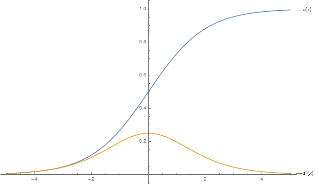
设数据集的特征维数为$n$,参数为$\theta = (\theta_1, \theta_2, \dots, \theta_n)$,则预测函数
\[h_{\theta}(x) = s(\theta^Tx) = \frac{1}{1+e^{-\theta^Tx}}\]表示对于输入$x$分类结果为类别$1$和类别$0$的概率:
\[\begin{cases} P(y=1\|x;\theta) &= h_{\theta}(x) \\ P(y=0\|x;\theta) &= 1 - h_{\theta}(x) \end{cases}\]损失函数
似然函数是一种关于统计模型参数的函数。给定输出$x$时,关于参数$\theta$的似然函数$L(\theta|x)$在数值上等于给定参数$\theta$后变量$X$的概率:
\[L(\theta\|x)=P(X=x\|\theta)\]在Logistic回归中,对于输入$x$的分类概率$P$可以表示为
\[P(y\|x;\theta) = (h_{\theta}(x))^y(1 - h_{\theta}(x))^{1-y}\]因此,似然函数:
\[L(\theta) = \prod_{i=1}^{m}P(y\|x_i;\theta)=\prod_{i=1}^{m}(h_{\theta}(x_i))^{y_i}(1 - h_{\theta}(x_i))^{1-y_i}\]对数似然函数:
\[l(\theta) = \log{L(\theta)} = \sum_{i=1}^{m}(y_i * \log{h_{\theta}(x_i))} + (1-y_i) * \log{(1 - h_{\theta}(x_i))}\]最大似然估计是求当$l(\theta)$的值最大时的参数$\theta$的值,取损失函数
\[J(\theta) = -\frac{1}{m}{l(\theta)}\]梯度下降法求解参数
梯度下降法更新$\theta$的过程:
\[\begin{aligned}\theta_j &= \theta_j - \alpha\frac{\partial{}}{\partial{\theta_j}}J(\theta) &= \theta_j - \alpha \frac{1}{m} \sum_{i=1}^{m}(h_{\theta}(x_i) - y_i)x_i^j \end{aligned}\]对于给定数据集,可以认为是有$m$条记录,$n$个特征的$m \times n$维矩阵$X$,训练数据集的分类结果是一个 长度为$m$的列向量$Y$,参数$\theta$是一个长度为$n$的列向量,将上述过程向量化,可得
\[\theta = \theta - \alpha X^T (s(X\theta) - Y)\]简单实现
m = 400      ## size of train set.
n = 300      ## number of features.
alpha = 0.1  ## learning rate

D = (rng.randn(m, n), rng.randint(size = m, low = 0, high = 2))
training_steps = 1000
x = T.dmatrix('x') ## input
y = T.dvector('y') ## output

## initialize weights
w = shared(rng.randn(n), name='w')

## initialize bias term, used to avoid overfitting.
b = shared(0., name='b')

# Construct Theano expression graph
p = 1 / (1 + T.exp(-T.dot(x, w) - b))        # Probability that target = 1
prediction = p > 0.5                         # The prediction thresholded
## xent = -y * T.log(p) - (1-y) * T.log(1-p)    # Cross-entropy loss function
## cost = xent.mean() ## + 0.01 * (w**2).sum()  # The cost to minimize
cost = T.nnet.binary_crossentropy(p, y).mean()
gw, gb = T.grad(cost, [w, b])                # Compute the gradient of the cost on w and b.

# compile
train = function(
        inputs=[x, y],
        outputs=[prediction, cost],
        updates=[(w, w - alpha * gw), (b, b - alpha * gb)])
predict = function(inputs=[x], outputs=prediction)

# train
for i in range(training_steps):
    pred, err = train(D[0], D[1])

# display arguments result:
# print(w.get_value(), b.get_value())

lables = D[1]            ## original labels.
classify = predict(D[0]) ## classify result using logistic regression.
ks = len([i for i in range(0, m) if D[1][i] != classify[i]])
print("correctness: ", (m-ks)/m)